Pseudogradient (Quasi-Newton) optimization techniques

Download Optimization.NET (.NET 6.0 / Nunit 3.0)

Both David-Fletcher-Powell (DFP) and BCFG algorithms belong to the group of the Pseudogradient (aka Quasi Newton)optimization algorithms. Pseudogradient methods are derived from gradient - based optimizations. These methods begin the search along a gradient line and use gradient information to build a quadratic fit to the model function. All of the algorithms involve a line search given by the following equation:

x_k+1 = x_k - aH_k Ñy(x_k)                               (1)

The line search in this context means finding a minimum of a one dimensional function defined by the gradient direction. For gradient search H_k is I, the unit matrix, and a is the parameter of the gradient line. For Newton's method H_k is the inverse of the Hessian matrix, H^-1; and a.

The Newton method works very well for the quadratic functions however, for nonlinear functions generally, Newton's method moves methodically toward the optimum, but the computational effort required to compute the inverse of the Hessian matrix at each iteration usually is excessive compared to other methods. Consequently, it is considered to be an inefficient middle game procedure for most problems. is one. For quasi-Newton methods H_k is a series of matrices beginning with the unit matrix, I, and ending with the inverse of the Hessian matrix, H^-1.

The DFP algorithm has the following form of equation (1) for minimizing the function y(x):
 

x_k+1 = x_k - a_k+1 H_k Ñy(x_k)                             (2)

where a_k+1 is the parameter of the line through x_k, and H_k is given by the following equation:

H_k = H_k-1 + A_k + B_k                                      (3)

The matrices A_k and B_k are given by the following equations.

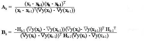(4) (5)

The algorithm begins with a search along the gradient line from the starting point x₀ as given by the following equation obtained from equation (6-13), with k = 0.

x₁ = x₀ - a₁H₀ Ñy(x₀)                               (6)

where H₀ = I is the unit matrix. The algorithm continues using equation (2) until a stopping criterion is met. However, for a quadratic function with n independent variables the method converges to the optimum after n iterations (quadratic termination) if exact line searches are used.

The matrices A_k and B_k have been constructed so their sums would have the specific properties shown below.

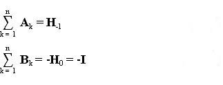(7) (8)

The sum of the n matrices A_k generate the inverse of the Hessian matrix H^-1 to have equation (3) be the same as Newton's method, equation (1), at the end of n iterations. The sum of the matrices B_k generates the negative of the unit matrix I at the end of n iterations to cancel the first step of the algorithm when I was used for H₀ in equation (6).

A further refinement of the DFP algorithm is the BFGS method which has been proven to have better convergence abilitied. The BFGS matrix up-date formula is:

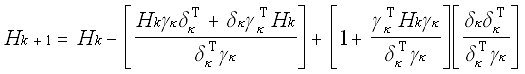    (9)

where d_k = x_k+1 - x_k and g_k = Ñy(x_k+1) - Ñy(x_k).

This equation is used in place of equation (3) in the algorithm given by equation (2). The procedure is the same in that a search along the gradient line from starting point x₀ is conducted initially according to equation (6). Then the Hessian matrix is updated using equation (9), and for quadratic functions the method arrives at the minimum after n iterations.